What are we aiming?
We aim to cluster the benzodiazepine use trajectories, in other words, check who maintained a low frequency use, who maintained a high frequency use, and maybe who changed their use frequency across the waves.
benzo_cld <- all_waves |>
    dplyr::mutate(id = as.character(dplyr::row_number())) |>
    dplyr::mutate(dplyr::across(dplyr::starts_with("benzofreq"), as.numeric)) |>
    dplyr::relocate(id,
                    benzofreq_w1, benzofreq_w2, benzofreq_w3,
                    dplyr::everything()) |>
    as.data.frame() |>
    kml::cld(timeInData = 2:4)

benzo_cld |>
    kml::kml()
#>  ~ Fast KmL ~
#> ***************************************************************************************************S
#> 100 S
long_col <- benzo_cld |>
    kml::getClusters(4) |>
    tibble::as_tibble_col("long_clust")

todo <- dplyr::bind_cols(all_waves, long_col) |>
    dplyr::mutate(dplyr::across(dplyr::starts_with("benzofreq"), as.numeric))


todo |>
    dplyr::group_by(long_clust) |>
    dplyr::summarise(dplyr::across(dplyr::matches("benzofreq_w[1-3]$"), mean))
#> # A tibble: 4 × 4
#>   long_clust benzofreq_w1 benzofreq_w2 benzofreq_w3
#>   <fct>             <dbl>        <dbl>        <dbl>
#> 1 A                  1.04         1.05         1.03
#> 2 B                  2.65         1.52         2.90
#> 3 C                  4.63         4.90         4.88
#> 4 D                  3.13         4.65         1.39
todo |>
    dplyr::group_by(long_clust) |>
    dplyr::count(benzofreq_w3) |>
    ggplot2::ggplot(ggplot2::aes(x = benzofreq_w3, y = n, fill = long_clust)) +
    ggplot2::geom_col()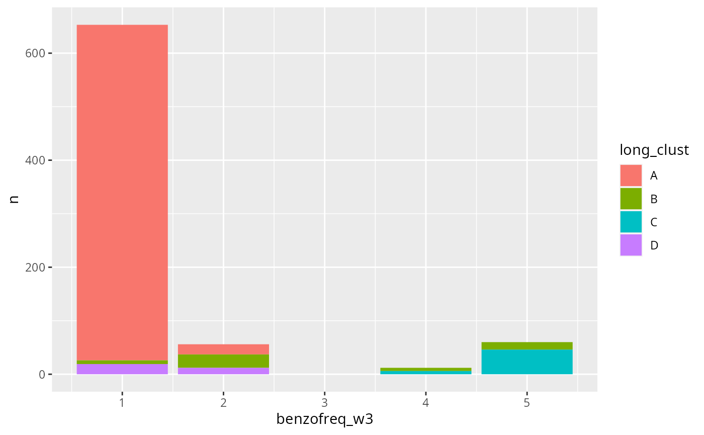
data_to <- todo |>
    dplyr::select(-dplyr::matches(".*w[2-3]$"), -benzofreq_w1)

data_to |>
    dplyr::count(long_clust)
#> # A tibble: 4 × 2
#>   long_clust     n
#>   <fct>      <int>
#> 1 A            646
#> 2 B             52
#> 3 C             52
#> 4 D             31

dados <- data_to |>
    dplyr::rename(trajectory = long_clust) |>
    dplyr::mutate(
        trajectory = relevel(as.factor(dplyr::case_when(
            trajectory == "A" ~ "Infrequente",
            trajectory == "B" ~ "Frequente",
            trajectory == "C" ~ "Redução de uso",
            trajectory == "D" ~ "Aumento de uso"
        )), ref = "Infrequente"),
        dplyr::across(c(dplyr::contains("relationship"), sleep_quality_w1),
                      \(x) as.factor(dplyr::case_when(
                          x %in% c("Ruim", "Ruins",
                                   "Regular", "Regulares") ~ "Worse",
                          x %in% c("Bom", "Bons",
                                   "Excelente", "Excelentes") ~ "Better",
                          x == "Não se aplica" ~ NA_character_,
                          TRUE ~ NA_character_)
                      )),
        household_income = as.factor(
            dplyr::case_when(
                household_income %in% c("A", "B") ~ "Upper",
                household_income %in% c("C") ~ "Middle",
                household_income %in% c("D", "E") ~ "Lower",
                TRUE ~ NA_character_
            )
        ),
        color = as.factor(
            dplyr::case_when(
                color %in% c("Parda", "Preta", "Amarela", "Indigena") ~ "Não-branco",
                color %in% c("Branca") ~ "Branco",
                TRUE ~ NA_character_
            )
        )
    ) |>
    dplyr::select(-state) |>
    dplyr::relocate(trajectory, dplyr::everything())