The idea
Considering that we have data on the frequency of benzodiazepine use for the three waves in these subjects (n = 781), we can try to create clusters referring to the pattern of use in these three moments through an unsupervised machine learning algorithm.
data("all_waves", package = "BenzoCovid")Clustering is a technique in machine learning that attempts to find clusters of observations within a dataset. The goal is to find clusters such that the observations within each cluster are similar to each other, while observations in different clusters are different from each other. So, we are not predicting a value based on a response/target variable, but instead, we are grouping the observations.
Feature transformation
The first step in this process is the transformation of the categorical variables of the frequency of use of benzodiazepines to numerical variables. This procedure is necessary because the k-means algorithm only accepts numerical features as input data.
We also took this step to select only the variables referring to the use of benzodiazepines in the subset of data.
3D scatterplot
Below is a 3D scatterplot showing the association between benzodiazepine use in the three assessment waves. In general, there is no great variation in the use frequency pattern in the sample.
plotly::plot_ly(
    benzo_frequencies,
    x = ~ benzofreq_w1,
    y = ~ benzofreq_w2,
    z = ~ benzofreq_w3,
    text = ~ paste(
        "Wave 1:",
        benzofreq_w1,
        "<br>Wave 2:",
        benzofreq_w2,
        "<br>Wave 3:",
        benzofreq_w3
    ),
    hoverinfo = "text"
) |>
    plotly::add_markers() |>
    plotly::layout(title = "Benzodiazepine Use Frequency in Each Wave",
                   scene = list(
                       xaxis = list(title = "Wave 1"),
                       yaxis = list(title = "Wave 2"),
                       zaxis = list(title = "Wave 3")
                   ))
K-means clustering
We start fitting three clustering models, from 1 to 5 clusters in order to find out the best number of clusters in our dataset.
set.seed(1)

benzo_kmeans <-
  tibble::tibble(k = 1:5) |>
  dplyr::mutate(
    kclust = purrr::map(k, ~kmeans(benzo_frequencies, .x)),
    tidied = purrr::map(kclust, broom::tidy),
    glanced = purrr::map(kclust, broom::glance),
    augmented = purrr::map(kclust, broom::augment, benzo_frequencies)
  )
Here, we can check which number of clusters behaves the best. We need to see the least amount of “distance” between the observations in the same cluster, and try to minimize the number of clusters used in order to keep a parsimonious model.
benzo_kmeans |>
  tidyr::unnest(cols = c(glanced)) |>
    ggplot2::ggplot(ggplot2::aes(x = k, y = tot.withinss)) +
    ggplot2::geom_line() +
    ggplot2::geom_point(size = 4, color = "darkslateblue") +
    ggplot2::theme_minimal(base_size = 20) +
    ggplot2::labs(title = "What's the optimal number of clusters?",
                  x = "# of clusters",
                  y = "Within sum of squares function") +
    gghighlight::gghighlight(k == 2)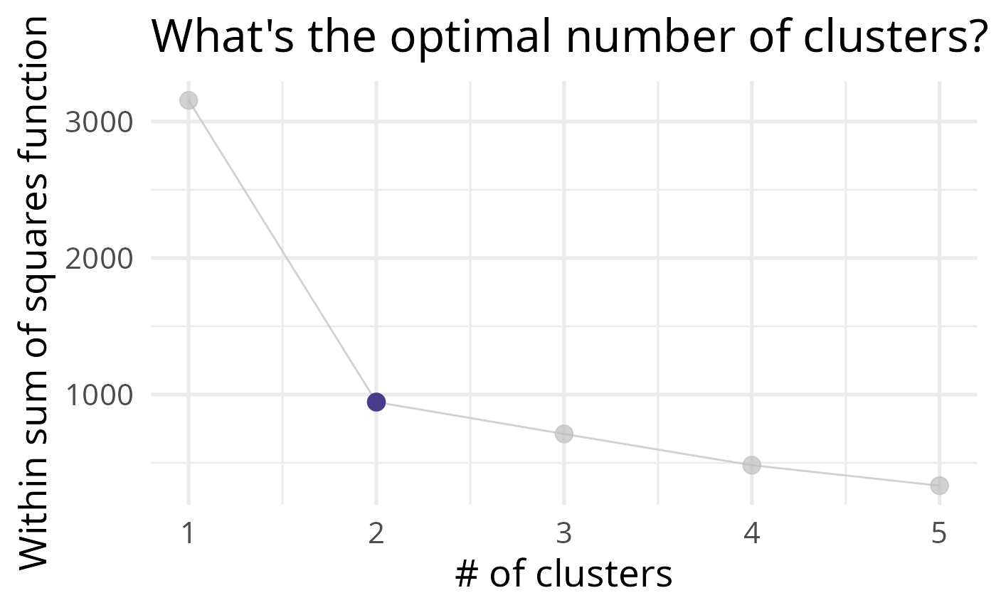
As we can see, this represents the variance within the clusters. It decreases as k increases, but notice a bend (or “elbow”) around k = 2. This bend indicates that additional clusters beyond the second have little value for us.
Now, we can see the mean values of each variable for each of the clusters. I have given myself the right to name the clusters as frequent use and infrequent use of benzodiazepines.
The frequent use cluster contains 86 subjects, and the infrequent use cluster contains 695 subjects.
two_clusters <- benzo_kmeans |>
    dplyr::pull(kclust) |>
    purrr::pluck(2)

two_clusters |>
    purrr::pluck("centers") |>
    base::as.data.frame() |>
    tibble::rowid_to_column("Cluster") |>
    dplyr::mutate(
        Cluster = dplyr::if_else(
            Cluster == 1, "Infrequent use",
            "Frequent use"
        )
    ) |>
    dplyr::rename(
        "Wave 1" = benzofreq_w1,
        "Wave 2" = benzofreq_w2,
        "Wave 3" = benzofreq_w3
        ) |>
knitr::kable(digits = 3, row.names = FALSE)| Cluster | Wave 1 | Wave 2 | Wave 3 |
|---|---|---|---|
| Infrequent use | 1.104 | 1.121 | 1.134 |
| Frequent use | 4.465 | 4.372 | 3.779 |
Join original data with cluster information
clustered_data <- two_clusters |>
    purrr::pluck("cluster") |>
    tibble::as_tibble_col("cluster") |>
    dplyr::mutate(cluster = dplyr::if_else(
        cluster == 1, "Infrequent", "Frequent"
    )) |>
    dplyr::bind_cols(all_waves)

utils::head(clustered_data)
#> # A tibble: 6 × 46
#>   cluster   age sex   color educa…¹ state region sexua…² heter…³ house…⁴ conta…⁵
#>   <chr>   <dbl> <fct> <fct> <fct>   <fct> <fct>  <fct>   <fct>   <fct>   <fct>
#> 1 Infreq…    47 Fema… Bran… Pós- g… São … Sudes… Hetero… sim     D       Não
#> 2 Freque…    34 Fema… Bran… Ensino… Rio … Sul    Bissex… não     D       Não
#> 3 Infreq…    57 Fema… Bran… Ensino… São … Sudes… Hetero… sim     B       Não
#> 4 Infreq…    52 Fema… Bran… Pós- g… Rio … Sul    Hetero… sim     A       Não
#> 5 Infreq…    32 Male  Bran… Ensino… Goiás Centr… Hetero… sim     D       Não
#> 6 Infreq…    44 Fema… Bran… Ensino… Rio … Sul    Hetero… sim     E       Não
#> # … with 35 more variables: risk_group_covid19 <fct>,
#> #   number_people_house <dbl>, benzofreq_w1 <fct>, benzofreq_w2 <fct>,
#> #   benzofreq_w3 <fct>, family_relationship_w1 <fct>,
#> #   family_relationship_w2 <fct>, family_relationship_w3 <fct>,
#> #   friend_relationship_w1 <fct>, friend_relationship_w2 <fct>,
#> #   friend_relationship_w3 <fct>, loving_relationship_w1 <fct>,
#> #   loving_relationship_w2 <fct>, loving_relationship_w3 <fct>, …
Is the pattern of suicidal ideation different between clusters?
BenzoCovid::grouped_count(clustered_data, "cluster", "suicidal_ideation_w1")
#> # A tibble: 4 × 3
#> # Groups:   suicidal_ideation_w1 [2]
#>   suicidal_ideation_w1 cluster        n
#>   <fct>                <chr>      <int>
#> 1 Yes                  Frequent      24
#> 2 Yes                  Infrequent    92
#> 3 No                   Frequent      62
#> 4 No                   Infrequent   603